Deploy a Flask App to Lightsail or other VS

Sudo apt update 
Sudo apt upgrade 
sudo apt-get -y install python3-pip 

If apt can’t find the module add the repository:

sudo add-apt-repository ppa:deadsnakes/ppa
sudo apt-get -y install python3-pip 

Install pipenv

pip3 install pipenv

Clone your repository

git clone https://github.com/account/myproject.git
cd project

Install the environment

pipenv install

I had problems with this and had to uninstall the apt vetrsion of virtualenv

sudo apt remove python3-virtualenv

Look for the green line under Creating virtual environment

Virtualenv location: /home/azureuser/.local/share/virtualenvs/myproject-qDDIoa4O

Make a note of that location

Configure Gunicorn

pipenv shell
pip install gunicorn
gunicorn --bind 0.0.0.0:5000 'myproject:create_app()'

in Azure and AWS port 5000 is blocked but you can create an ssh tunnel to test to make sure your app is working:

#Local Terminal
ssh -N -L 5000:127.0.0.1:5000 <server ip>

in a browser go to http://127.0.0.1:5000/ and your app should pop up.

ctrl-c to terminate the gunicorn process

exit

to leave the virtual environment

vim  /etc/systemd/system/myproject.service 

[Unit]
Description=Gunicorn instance to serve myproject
After=network.target

[Service]
User=ubuntu
Group=www-data
WorkingDirectory=/home/ubuntu/myprojectdir
Environmment="PATH=/home/ubuntu/.local/share/virtualenvs/myproject-8Mk7vn
ExecStart=/home/ubuntu/.local/share/virtualenvs/myproject-8Mk7vntI/bin/gunicorn --workers 3 --bind unix:myproject.sock -m 007 myproject:create_app()

[Install]
WantedBy=multi-user.target

Start and enable service:

sudo systemctl start myproject
sudo systemctl enable myproject

Configure Nginx

If nginx isn’t installed

sudo apt install nginx
sudo vim /etc/nginx/sites-available/myproject

i to insert

server {
    listen 80;
    server_name your_domain www.your_domain;

    location / {
        include proxy_params;
        proxy_pass http://unix:/home/ubuntu/myproject/myproject.sock;
    }
}

esc then :wq to write and quit

Link your site in available to sites-enabled

sudo ln -s /etc/nginx/sites-available/myproject /etc/nginx/sites-enabled

run test

sudo nginx -t

Restart nginx

sudo systemctl restart nginx

Test from your browser that it’s working

Add SSL

https://certbot.eff.org/instructions?ws=nginx&os=ubuntufocal

ensure snap is installed

sudo snap install core; sudo snap refresh core

use snap to install certbot

sudo snap install --classic certbot

link the certbot to bin

sudo ln -s /snap/bin/certbot /usr/bin/certbot

Run certbot

sudo certbot --nginx

follow instructions and you’re set.

Running into Problems

One way to diagnose potential problems is to view the terminal journal of the service

journalctl -u <app name>

Running old wordpress themes on Lightsail

I do not recommend continuing to use PHP 5.6. It’s full of vulnerabilities, but I needed to buy myself some time with some old WordPress themes that error out on higher version of php.

Stop bitnami services and save the instance as a backup

sudo /opt/bitnami/ctlscript.sh stop
sudo mv /opt/bitnami /opt/bitnami.back

Download and install archived instance (check the Bitnami changelog to find if you need a different version, then just update the numbers accordingly)

cd /tmp
curl -LO https://downloads.bitnami.com/files/stacks/wordpress/4.8.2.php56-0/bitnami-wordpress-4.8.2.php56-0-linux-x64-installer.run

chmod +x bitnami-wordpress-4.8.2.php56-0-linux-x64-installer.run
sudo ./bitnami-wordpress-4.8.2.php56-0-linux-x64-installer.run

for PHP 7 useupl

 curl -LO https://downloads.bitnami.com/files/stacks/wordpress/5.9.1-0/bitnami-wordpress-5.9.1-0-linux-x64-installer.run

The newest version (at writing) using PHP8 is 6.1.1-0 and can be downloaded:

curl -LO https://downloads.bitnami.com/files/stacks/wordpress/6.1.1-0/bitnami-wordpress-6.1.1-0-linux-x64-installer.run

install to /opt/bitnami/

sudo nano /opt/bitnami/apache2/conf/bitnami/bitnami.conf

update document root

DocumentRoot "/opt/bitnami/apache2/htdocs"
  <Directory "/opt/bitnami/apache2/htdocs">

to

 DocumentRoot "/opt/bitnami/apps/wordpress/htdocs"
  <Directory "/opt/bitnami/apps/wordpress/htdocs">

then lower under ssl

<VirtualHost _default_:443>
  DocumentRoot "/opt/bitnami/apps/wordpress/htdocs"  #Edit
  SSLEngine on
SSLCertificateFile "/opt/bitnami/apache2/conf/server.crt"
SSLCertificateKeyFile "/opt/bitnami/apache2/conf/server.key"

  <Directory "/opt/bitnami/apps/wordpress/htdocs"> #Edit

...

at the end add the following to allow for larger PHP uploads. Adjust so your All-in-One WordPress Backup file will upload.

php_value upload_max_filesize 128M
php_value post_max_size 128M
php_value memory_limit 256M
php_value max_execution_time 300
php_value max_input_time 300

sudo nano /opt/bitnami/apps/wordpress/htdocs/wp-config.php

define('WP_SITEURL', 'http://' . $_SERVER['HTTP_HOST'] . '/wordpress');
define('WP_HOME', 'http://' . $_SERVER['HTTP_HOST'] . '/wordpress');

to

define('WP_SITEURL', 'http://' . $_SERVER['HTTP_HOST]);
define('WP_HOME', 'http://' . $_SERVER['HTTP_HOST']);

sudo nano /opt/bitnami/apache2/conf/bitnami/bitnami-apps-prefix.conf

#Include "/opt/bitnami/apps/wordpress/conf/httpd-prefix.conf"  

sudo /opt/bitnami/ctlscript.sh restart apache

go ahead and enter ip address in browser

Update WordPress and plugins

Before using all-in-one wp migration change the a record to the new ip address and set up encryption.

https://docs.bitnami.com/aws/how-to/generate-install-lets-encrypt-ssl/

Install Let’s Encrypt

For bitnami v5.9.1 just run

sudo /opt/bitnami/bncert-tool

For older versions, you’ll have to install the tool first

wget -O bncert-linux-x64.run https://downloads.bitnami.com/files/bncert/latest/bncert-linux-x64.run
sudo mkdir /opt/bitnami/bncert
sudo mv bncert-linux-x64.run /opt/bitnami/bncert/
sudo chmod +x /opt/bitnami/bncert/bncert-linux-x64.run
sudo ln -s /opt/bitnami/bncert/bncert-linux-x64.run /opt/bitnami/bncert-tool

now you can run the Bitnami HTTPS Configuration Tool

sudo /opt/bitnami/bncert-tool

Remove Bitnami Banner

sudo /opt/bitnami/apache2/bnconfig --disable_banner 1

Reverse Order Numbering in Microsoft Word

  1. Select Paragraphs
  2. Under insert, click Table, then Convert Text To Table…
  3. Number of Columns: 1
  4. Separate Text at: Paragraph
  5. Click Ok
  6. Right-click on table -> Insert -> Columns to the Left
  7. Shrink column size by dragging middle boundary toward left
  8. With ONLY left column selected, under Home, click Numbering (numbered list)
  9. Copy all numbers
  10. Open new document, and Paste as “Keep Text Only”
  11. Under Home, click Sort (a -z with an arrow)
  12. Sort by: Paragraphs, Descending
  13. Click ok
  14. Copy Text
  15. In original document, with original numbers selected, under Home, click Numbering(number list) to turn off numbering
  16. Ctrl-v or paste your sorted list of numbers.
  17. Format table by right clicking on table edge and selecting Table Properties

Thanks to Susan Harkins from techrepublic.com for the Original Post

Using IF ELSE in R

Basics:

x <- 5
if (x == 5){ 
   print("x = 5")
   }
#response: "x = 5"

if (x == 6){
   print("x = 5")
}
#no response

If Else

if (x == 5){
   print("x = 5")
 }else{
   print("x doesn't equal 5")

 }
#response "x = 5"

if (x == 6){
  print("x = 6")

}else{
  print("x doesn't equal 6")
}
#response: "x doesn't equal 6"

To make a IF NOT statement add the ! function in the mix

x <- 5
if (!(x == 5)){ 
   print("x does not = 5")
   }
#no response

if (!(x == 6)){ 
   print("x does not = 6")
   }
#response: "x does not = 6"

For numbers you can do the same thing with the not equal sign

x <- 5
if (x != 6){ 
   print("x does not = 6")
   }
#return "x does not = 6"

Make a chain of if statements with if, else if statements. (like python’s elif)

x <- 5
if (x < 5){ 
   print("x is less than 5")
   }else if(x > 5){
     print("x is more than 5")
   }else if(x == 5){
     print ("x is equal to 5")
   }else {
     print ("x is not a number")
   }
#return: "x is equal to 5"

Also look at elseif()

ifelse returns a value with the same shape as test which is filled with elements selected from either yes or no depending on whether the element of test is TRUE or FALSE.

x <- 5
print(ifelse(x==5, 'x is equal to 5', NA))
# "x is equal to 5"

print(ifelse(x==6, 'x is equal to 5', 'x is not equal to 5'))
# "x is not equal to 5"

ifelse(x == 5, print('x is equal to 5'), print('x is not equal to 5'))
# "x is equal to 5"
# "x is equal to 5"

y <- 5
ifelse(y == 5, print('y is equal to 5'), print('y is not equal to 5'))
# "y is not equal to 5"

NOTE: ifelse() strips attributes

https://rdrr.io/r/base/ifelse.html

For Tidyverse look at if_else()

https://dplyr.tidyverse.org/reference/if_else.html

Tapered Stream Lines from NHD Plus HR in ArcGIS Pro

Download NHDPlus HR Data

You can find the Data on the National Map:

https://apps.nationalmap.gov/downloader/

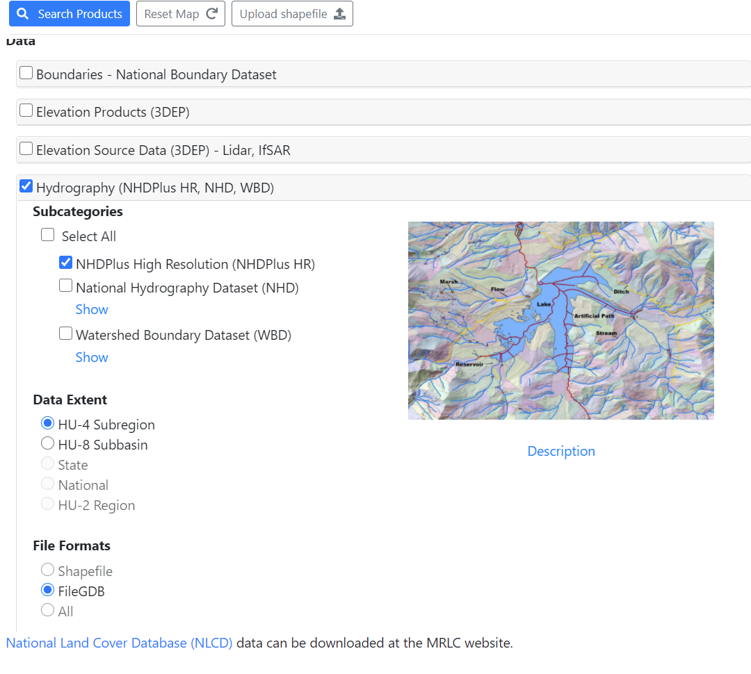
Zoom into the area you need data for, check Hydrography, NHDPlus High Resolution, then HU-4 Subregion (HUC 4 areas) unless you need a smaller area then HU-8.

Click the big blue button Search Products

Download the products you need. Choose the “Zip” version which is the GDB. If you get the z7 version you’ll download the Raster version.

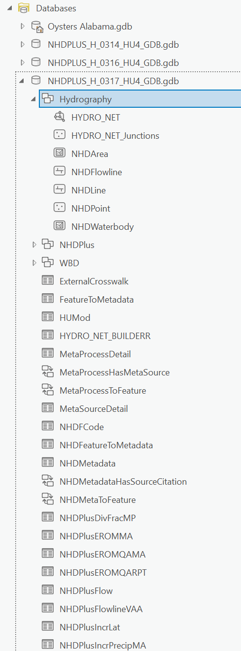
Once downloaded, unzip, then drag the GDB folder to the database folder in the Catalogue panel.

Under Hydrography, drag NHDFlowline to your contents panel, then drag the NHDPlusFlowlineVAA table to contents as well.

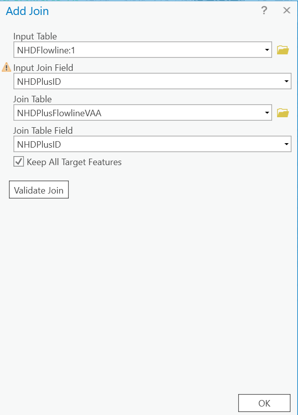
On Contents panel, right click on NHDFlowline, under Joins and Relates, click Add Join.

for input Join Field, select NHDPlusID.
For Join Table, select NHDPlusFlowlineVAA then add NHDPlusID to the Join Table Field if it doesn’t auto populate.

Now that the polypath has the data we need, right click NHDFlowline in Contents panel and select Symbology to open its panel.

When I first started working with tapered streams, I would use “Mean Flow Volume,” but I’ve found using the TotalDrainageAreaSqKm creates better results especially for delta areas where rivers split.

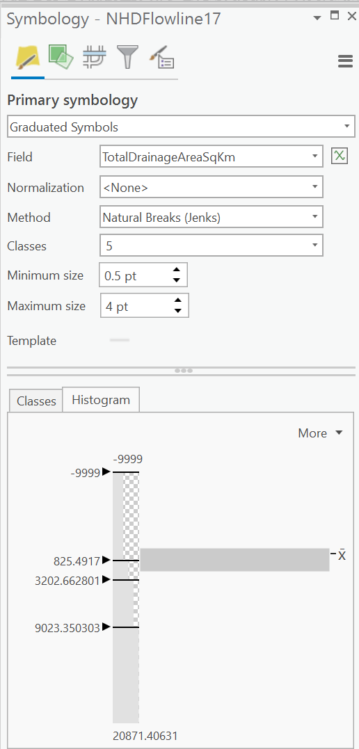
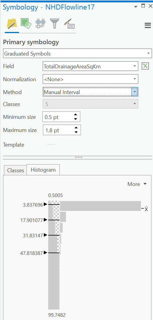
In the Symbology panel, select TotalDrainageAreaSqKm then take a look at the Histogram

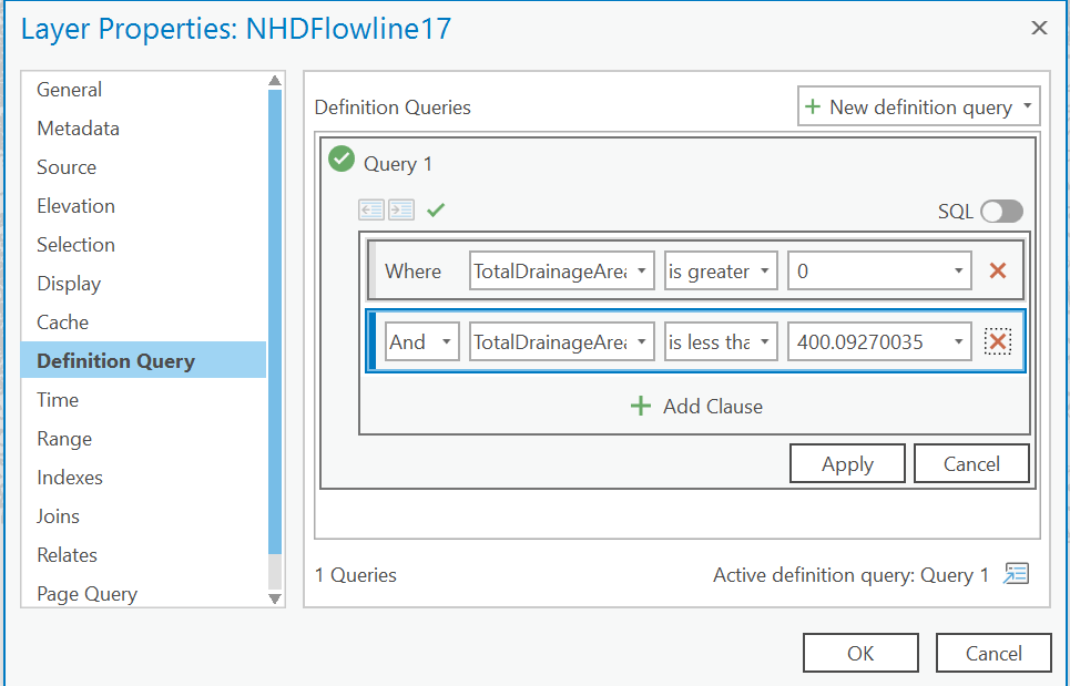
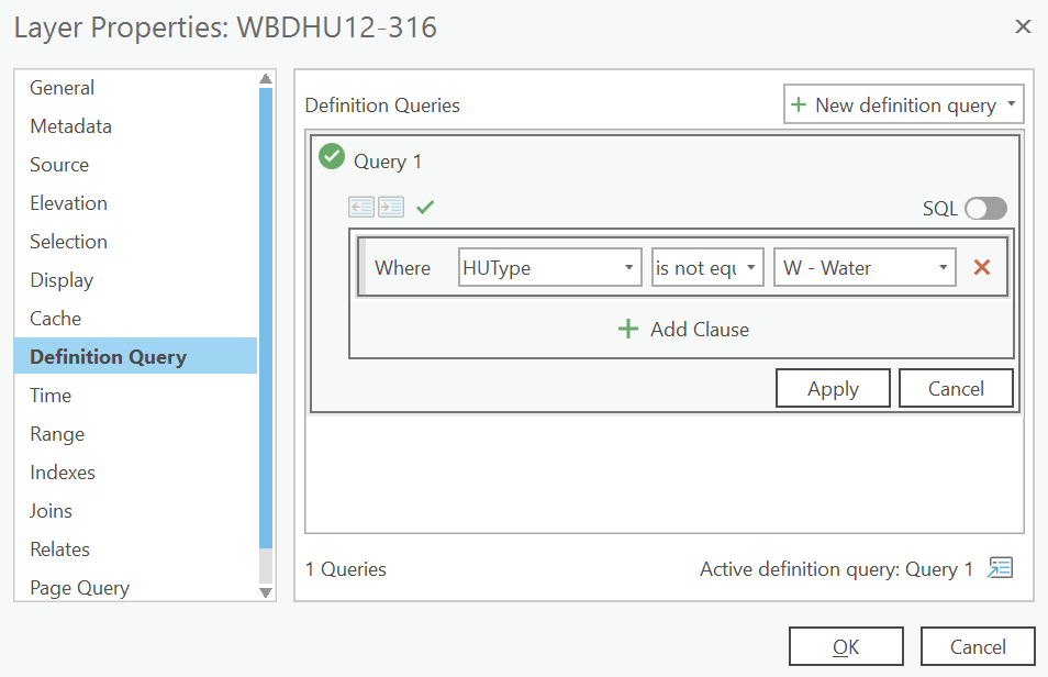
It looks like there are values in the -9999 (likely meaning a stream segment without information available), then a tiny percentage of streams with the largest area. To fix this, double click on NHDFlowline in Contents panel to open its properties. Select Definition Query, hit the +, and add a new query Where upstreamCumulativeAreaSqKm is greater than 0 AND UpstreamCumulativeAreaSqKm is less than 400.

Now when you pull up the Histogram in Symbology, it will present something much more meaningful.

Set Classes to 5, switch to Manual Interval, then adjust the Histogram breakpoints until it look right.

Now we’ve got to add back those major trunk rivers. Right click on NHDFlowline, click copy, then right click on the map name at the top (unless you renamed it it may be “Map”) select Paste. Rename this feature set by clicking on the words once. Change its name to NHDFlowlineBigRiver

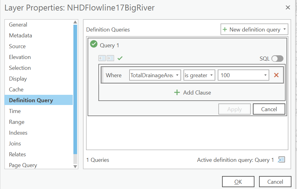
Double click to enter its properties, select Definition Query. Then edit the definition Where TotalDrainageArea is greater or equal to 100 .

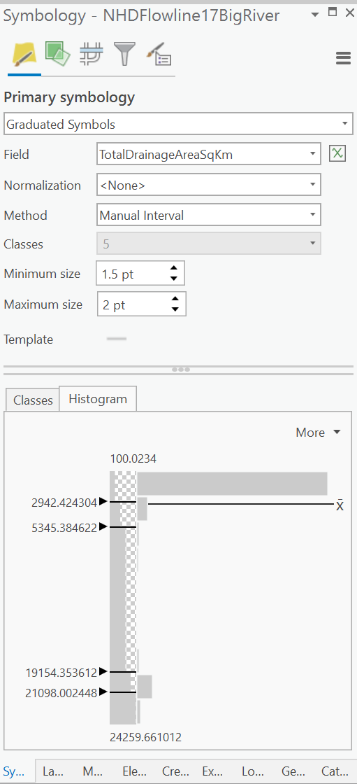
Go back to your Symbology panel, create 5 classes between 1.5 and 2pt, then change adjust values in histogram as needed.

Part 2 coming soon.

ArcGIS sketch to Lat Long

I’m sure there’s a better way to convert a sketch layer into coordinates, but this worked for me.

Use Geoprocessing tool: Layer to KML

Then use KML to Layer to import it back in with the coordinate system the map is in.

Open the features table, calculate:

New field: Lon

Lon = shapeToY(!Shape!)

Code Block:

def function(shape):
   point=shape.getPart(0)
   return point.Y

Repeat for the calculation for x

Data Sources

One of the most time-consuming parts of building maps is finding the data sets you want. I’m often forgetting where I found different datasets, and I wanted to share some of the ones I like to go back to.

USA Datasets

USGS National Map

https://apps.nationalmap.gov/viewer/

Mineral Resources Online Spatial Data:

https://mrdata.usgs.gov/general/map-us.html

Purdue’s GIS Data by State

A concise list of important resources available to you on the web and at Purdue. https://guides.lib.purdue.edu/c.php?g=353290&p=2378621

Convert DDMM.SS to Decimal Degrees

Quick tip if you get data coded with your lat long coded in Deg, Min, Sec

Open your table -> Calculate Field -> New Field = Lat
Field Type = Float
Lat = ConvertLat(!START_LAT__DDMM_MM_!)

def ConvertLat(lat):
    d = lat[-7:-5]
    m = lat[-5:-3]
    s = lat[-2:]
    return float(d) + float(m)/60 + (float(s)/(60*60))

Do the same thing for Long, keep in mind you may need to add a “-” to your calculation.

Field Name = Lon
Field Type = Float
Lon = ConvertLat(!START_LON__DDMM_MM_!)

def ConvertLat(lon):
    d = lon[-7:-5]
    m = lon[-5:-3]
    s = lon[-2:]
    return -(float(d) + float(m)/60 + (float(s)/(60*60)))

if your decimal is DD MM.MMM then you can use

def ConvertLat(lat):
    d = lat[:2]
    m = lat[3:8]
    return float(d) + float(m)/60

Don’t forget to add – if W or S

def ConvertLat(lon):
    d = lat[:2]
    m = lat[3:8]
    return -(float(d) + float(m)/60)

Custom Bathymetry with Labeled Contours ArcGIS Pro

Download a Digital Elevation Model (DEM) of the area of interest from NOAA.

https://www.ncei.noaa.gov/maps/bathymetry/

Filter only by DEM Footprints. I’m going to use the Northern Gulf of Mexico 1 arc-second.
Click the link for the metadata then download the NetCDF file (750MB).

ArcGIS doesn’t work natively with NC files, so from the View ribbon, click Geoprocessing button to open the Geoprocessing panel, search for Make NetCDF Raster Layer

Input NetCDF File: northern_gulf_1_navd88_.nc

Use the defaults for the next three options
Variable: Band 1
X Dimension: lon
y Dimension: lat
Change the Output Raster Layer something more descriptive: NorthernGulfDEM
Leave the other defaults:

This can take a few minutes to process but when it’s done the new raster layer will have the Bathymetry color scheme.

This section covers way more area than I need, so I’m going to crop it using the Intersect tool so future changes won’t require as much processing power.

Create Feature Layer and Cropping Polygon

First create a feature layer.

Open Catalogue pane (View ribbon, Windows section)
Expand Databases
Right-click on the home database (TrainingMap.gdb) go into New, then select Feature Class

Name the new class
Name: CroppingPolygon
Alias: Cropping Polygon
Type: Polygon
M Value: Unchecked
Z Value: Checked
Add output dataset to current maps: Checked

Hit Next, then add a new Field
Field Name: Name
Data Type: Text

Hit Next
On the Spatial Reference page, make sure you are using the coordinate system you are using on the rest of the map.

Hit Next
Keep defaults on the Tolerance page
XY Tolerance: 0.001
Z Tolerance: 0.001

Hit Next and keep defaults on the Resolution page

Hit Next and keep defaults on Storage Configuration, then hit Finish.

From Edit ribbon, Features section, click the Create button to open the Create Feature panel

Double-click Cropped Polygon, and select the Rectangle tool

The Rectangle Tool works by clicking the top left point of your rectangle, then clicking the top right point of your rectangle, then clicking the bottom right corner of the rectangle.

Hit the green check mark at the bottom of your map, then click the Save button on the Edit ribbon to save this new polygon to the database. ArcGIS then asks, “Save all edits?” Click yes.

In the Contents panel, right-click on the Cropped Polygon layer and open the Attributes Table.
Double click <null> in the name column of the entry for the new polygon and give it a descriptive name: Mobile Bay Area.

Click the Save button again from the Edit ribbon.

Cropping with the Clip Raster tool

From the View ribbon, select Geoprocessing to open the Geoprocessing panel
Search for Clip Raster and double-click to open the Clip Raster panel

In the parameters page:
Input Raster: NorthernGulfDEM
Output Extent: Cropped Polygon,
Leave the Rectangle options
Output Raster Dataset: NorthernGulfDEM_Clip_MobileBay
Check Maintain Clipping Extent (otherwise, you’ll end up getting a different section of the image)
Click Run

From Contents panel, uncheck both the Cropped Polygon and NorthernGulfDEM layers.

Create Contours from DEM

From the View ribbon, select Geoprocessing to open the Geoprocessing panel
Type into the search “Contour” then open the Contour (3d Analyst Tools)

On the Parameters page of the Contour tool, set the following values:
Input raster: NorthernGulfDEM_Clip_MobileBay
Output: Contour_MobileBay
Contour Interval: 10 (assumed Meters because in Map properties, on the general tab, the Map Units are set to Meters)
Base contour: 0
Z factor: 1 (change this if converting meters to feet, etc)
Contour Type: Contour

Simplify Contour

NOTE: you may need to run DEFINE PROJECTION geoprocessing tool on the contours before simplifying.

Open the Geoprocessing Panel (from View ribbon)
Search for Simplify Line, and open it.

From the Parameters page set the following values:
Input Feature: Contour_MobileBay
Output Feature Class: Contour_Simplify_MobileBay
Simplification Algorithm: Retain critical bends (Wang-Müller)
Simplification Tolerance: 1 Kilometers
Uncheck “Keep collapsed points”
Input Barrier Layers: <blank>
Click Run (this may take a while, be glad the original DEM is clipped!)

If you get an error: The cartographic spatial reference does not have a projected coordinate system,
Use the Define Projection tool to set a projection for your input contour feature.

The results look better, but there’s still too many artifacts. Use the Definition Query to clean this up.

In Contents panel Double-click on Contour_Simplify_MobileBay to open its Property panel then navigate to the Definition Query page
Hit + New Definition Query
Set Query 1 to Where Shape_Length is greater than 0.1

That’s much better!

Create Labels for Contours

The new contours still need labels.

In the Contents panel, right-click on the new Contour_Simplify_MobileBay and select Label to turn on labels
Right-click on the feature again and select Label Properties to open the Label Class Properties panel
Delete contents of Expression box, then double-click on Contour in Fields to add it to the expression.
Click Apply.

Click on the Position tab
Open up Placement, and change Regular placement to Contour placement
Chose Page label alignment
Adjust “Maximum label angle” to something above 30°
Uncheck “Place labels in ladders” (unless you prefer all the labels to line up)
Click Apply

On the Symbols tab of the panel, open Appearance
Font name: Arial
Font style: Regular
size: 10pt
Text fill symbol: leave default
Color: Gray 10%
Open up Halo
Halo Symbol: White Fill
Color: Use the eyedropper to click anywhere in the water to select the color of the background. 
Halo size: 2pts
Click Apply

We’ll revisit these settings after we decide what our water will look like.

Create Contours with Contour Raster Function

To get intermediate unlabeled contours, select Raster Functions panel (Analysis ribbon, Raster section)

Type in Contour and select the Contour tool

Raster: NorthernGulfDEM_Clip_MobileBay
Adaptive Smoothing : 2.5 (default)
Contour Type: Contour lines
Z Base: 0
Number of Contours: 0
Contour Interval: 1
Z Factor: 1
Click Create new layer

In the contents panel, drag this layer below Contour_MobileBay_Simplify

This is way to busy, to change the color of the intermediate contour lines, right-click on Contour_NortherGulfDEM_Clip select Symbology to open the Symbology panel
From Color Scheme select Format Color Scheme shown below the list of gradients

In the Color Scheme Editor, click on the l black box on the left side of the gradient to make it active
Either change the color to something with less contrast or set the transparency to 80%
Click OK to apply the new color.

That’s looking better. Change the color of the labeled contour by double-clicking on the line icon under Contour_Simplify_MobileBay in the Contents panel, then switch to the Properties tab
Open the color picker and chose Color Properties below the Eyedropper.

Color Model: HSL (This turns the sliders into Hue, Saturation, Lightness, and Transparency)
Drag the saturation slider left to 0%
Drag darkness left to around 50%
Finally, drag transparency right to around 30%
Click OK, then click Apply in the Symbology panel

Create Buffer Mask for Contour Labels

Once size and location of labels looks correct, in Contents panel, right-click on your contour layer, and select Convert Labels -> Covert Labels to Annotations

Double-check your Conversion Scale, select your geodatabase, click run.

Open Buffer from Geoprocessing Tools -> Spatial Analyst Tools

Input Feature: your annotation layer

Distance: 1 Point

Hide layer.

From Contents panel select your contour label.

From Feature Layer Ribbon, select your buffer label.

Quickly Transform Text Values to Numbers in ArcGIS Pro with Python If statement

If you have a table with values of text that you want to change into numeric values to manipulate symbology, you can use the Python Code Block in the Calculate Field tool.

I want to add a column of numbers to correspond to these text descriptions

Non-detect -> 1
Low -> 1
Moderate -> 2
High -> 3
Very High -> 4

To do this, I’ll open the table in ArcGIS Pro, then click the Calculate button to open the Calculate Field Panel

In Calculate Field, chose the the table you want to edit, add a new field for your numbers “riskNumbers,” then make that a Long Integer field.

After the “=” add the code:

makeNumbers(!riskName!)

Then in the Code Block Section we’ll define our makeNumbers function:

def makeNumbers(risk):
    if risk == 'Non-detectable':
        return 0
    elif risk == 'Low':
        return 1
    elif risk == 'Moderate':
        return 2
    elif risk == 'High':
        return 3
    elif risk == 'Very High':
        return 4

Check your new RiskNumber column and spot check to make sure it worked.

Now you can go on to add gradient symbology to your data.